Week 8: Geostatistics–Kriging
1 Introduction
- In this Lab, we will learn two key functions
- krige.control: specify parameters for kriging, no computing involved.
- krige.conv: to compute
- Usage
- krige.control(type.krige = “ok”, obj.model = NULL)
- Type of kriging: “sk”, “ok” (default)
- obj.model: typically an output of likefit
- Usage
- krige.conv(geodata, locations, krige)
- geodata
- locations: \(\mathbf s_0\), data.frame, multiple locations.
- krige: output of krige.control.
2 Ordinary Kriging
First, we fit the model \[Z(\mathbf{s}) = \mu + U(\mathbf{s}) + \nu(\mathbf{s}).\] Here trend = “cte” specifies that the trend \(\mu(\mathbf{s})\) is a constant (\(\mu(\mathbf{s})=\mu\)).
library(geoR)
data(ca20)
fit = likfit(ca20, ini = c(100, 120), trend = "cte")
Secod, we setup the Ordinary Kriging.
pred_locs = expand.grid(x = seq(5300, 5800, 10), y = seq(5000,5600, 10))   # new locations s_0 created
head(pred_locs)     ## Here are the first six locations
## x y
## 1 5300 5000
## 2 5310 5000
## 3 5320 5000
## 4 5330 5000
## 5 5340 5000
## 6 5350 5000KC = krige.control(obj.model = fit)If you want to know what expand.grid does, try
#tmp = expand.grid(x = 1:10, y = 1:5)
#plot(tmp)
Third, we make predictions on all locations on pred_locs
ca20pred = krige.conv(ca20, loc = pred_locs, krige = KC)- The output includes
- ca20pred$predict: the kriging estimates for all locations specified at loc.
- ca20pred$krige.var: the kriging variance for all locations specified at loc.
Last, we visualise both Kriging estimates and Kriging variances. The function to use is geom_tile
ca20_res = data.frame(x = pred_locs[,1], y = pred_locs[,2],
                      krige = ca20pred$predict, krige_var = ca20pred$krige.var)


library(ggplot2)
ggplot(ca20_res) + geom_tile(aes(x = x, y = y, fill = krige))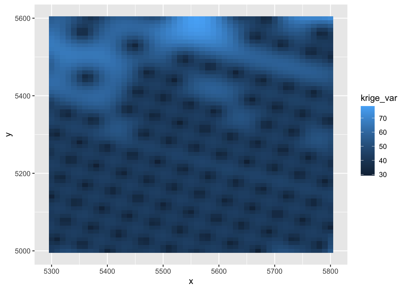
Kriging Variances
p1 = ggplot(ca20_res) + geom_tile(aes(x = x, y = y, fill = krige_var))

p1
3 Universal Kriging
Both ordinary kriging and universal kriging using setting type.krige = “ok”. Once you put the trend in, the function will distinguish two types of kriging.
3.1 Universal Kriging: Polynomial of coordinates
- We need to provide \(x_1(\mathbf s_0),
\ldots, x_p(\mathbf s_0)\) for the function
- in function krige.control
- trend.d: specify data trend
- trend.l: specify prediction trend
Work with polynomial.
fit = likfit(ca20, ini = c(100, 60), trend = "1st")
KC = krige.control(obj.model = fit, trend.l="1st",
                   trend.d="1st")
ca20pred = krige.conv(ca20, loc = pred_locs, krige = KC)
3.2 Universal Kriging: covariates
fit2 = likfit(ca20, ini = c(100, 60), trend = ~altitude)
graltitude = rnorm(3111,mean=5.5)
KC2 = krige.control(type.krige = "ok", obj.model=fit2,
                    trend.d=~altitude, trend.l=~graltitude)
ca20pred2 = krige.conv(ca20, loc = pred_locs, krige = KC2)
In universal kriging, we need to know \(x(\mathbf s_0)\). In the above code, I randomly generated \(x(\mathbf s_0)\) from graltitude = rnorm(3111,mean=5.5). In practice, you shall know \(x(\mathbf s_0)\) in advance.
4 Kriging weights
coords = cbind(c(0.2, 0.25, 0.6, 0.7),
               c(0.1, 0.8, 0.9, 0.3))   # data
KC = krige.control(ty = "ok", cov.model = "mat",
                   kap = 1.5, nug = 0.1,
                   cov.pars = c(1, 0.1))    # model parameter
# Weights
krweights(coords, c(0.5, 0.5), KC)
## [1] 0.1935404 0.2301559 0.2125838 0.36371995 Exercise
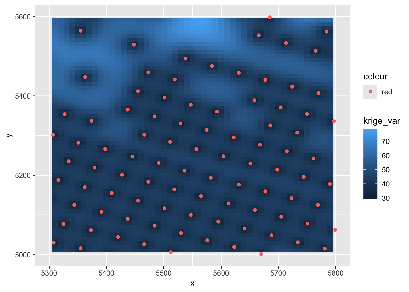
The observed locatins are plotted over the kriging variance. Do you see any pattern?
obs_locations = data.frame(ca20$coords)

p1 + geom_point(data = obs_locations, aes(x = east, y = north, col = "red")) + xlim(5300, 5800) + ylim(5000,5600)