Week 5: Visualisation of Spatial Data (2) – sf
Here, sf (simple feature) is a type of data class. First, we use package sf to read shapefiles.
1 Shapefile
- A shapefile is a simple, nontopological format for storing the
geometric location and attribute information of geographic features. It
is developed by Esri (Environmental Systems Research Institute, the
company that makes famous ArcGIS software). It usually includes the
following file
- .shp: geometries
- .shx: an index file to the geometries
- .dbf: storing attribute data
- The shapefile here is named Aus-Melbourne02, which records
information from all LGA in Greater Melbourne.
- All datasets can be downloaded at https://github.com/TedChu/90122Lab/tree/master/datasets or in Files – datasets (LMS)
- First, set the working directory through setwd. Remember you need to use forward-slash (/) or double slash (\\), but NOT backslash (\).
- I will not recommend you to have space between your folder titles. That is, to write setwd(“…./90122Lab”), Not setwd(“…./90122 Lab”)
- Depending on where you store your files, you need to adjust directories in setwd and dsn.
library(sf)
gmel = st_read(dsn = "datasets/Mel/Aus-Melbourne02.shp", "Aus-Melbourne02")
## Reading layer `Aus-Melbourne02' from data source
## `/Users/tingjinc/Library/CloudStorage/OneDrive-TheUniversityofMelbourne/2_MAST90122/90122LabGit/datasets/Mel/Aus-Melbourne02.shp'
## using driver `ESRI Shapefile'
## Simple feature collection with 32 features and 14 fields
## Geometry type: POLYGON
## Dimension: XY
## Bounding box: xmin: 144.444 ymin: -38.49937 xmax: 146.1925 ymax: -37.40175
## Geodetic CRS: WGS 84The object gmel belongs to the sf class, which extends the data.frame class. Note that the last column is called geometry, which stores the shape of the region.
class(gmel) ## [1] "sf" "data.frame"print(gmel[1:3], n = 3)## Simple feature collection with 32 features and 3 fields
## Geometry type: POLYGON
## Dimension: XY
## Bounding box: xmin: 144.444 ymin: -38.49937 xmax: 146.1925 ymax: -37.40175
## Geodetic CRS: WGS 84
## First 3 features:
## id country name geometry
## 1 4246124 AUS Greater Melbourne POLYGON ((144.444 -37.86413...
## 2 2403625 AUS City of Banyule POLYGON ((145.0278 -37.7638...
## 3 3333042 AUS City of Bayside POLYGON ((144.9838 -37.9028...2 Manuplation of sf object
You can manipulate the sf object similar to a data.frame object. Here, I want to remove the first element since it is greater Melbourne, not LGA.
gmel = gmel[-1,] # the first element is greater melbourne, not LGAR package mapview provides functions to create interactive visualisation of spatial data.(For more details, please see “https://r-spatial.github.io/mapview/index.html”). A simple interactive map can generated as below.
library(mapview)
mapView(gmel)
Variables
gmel$name # Extracting a variable## [1] "City of Banyule" "City of Bayside"
## [3] "City of Boroondara" "City of Brimbank"
## [5] "City of Casey" "City of Hume"
## [7] "City of Darebin" "City of Frankston"
## [9] "City of Glen Eira" "City of Greater Dandenong"
## [11] "City of Hobsons Bay" "City of Kingston"
## [13] "City of Knox" "City of Manningham"
## [15] "City of Maribyrnong" "City of Maroondah"
## [17] "City of Melbourne" "City of Melton"
## [19] "City of Monash" "City of Moonee Valley"
## [21] "City of Moreland" "City of Port Phillip"
## [23] "City of Stonnington" "City of Whitehorse"
## [25] "City of Whittlesea" "City of Wyndham"
## [27] "City of Yarra" "Shire of Cardinia"
## [29] "Shire of Mornington Peninsula" "Shire of Nillumbik"
## [31] "Shire of Yarra Ranges"gmel$ID = 1:31 # Add a new variable
gmel$ID = NULL # Delete a variableSelect LGA == City of Banyule is
i = which(gmel$name == "City of Banyule")
g = gmel[i, ]
mapView(g)
3 Combining Data (Optional)
LGA information based on 2015 survey are available in LGAData.csv. It includes around 400 variables.
- Here, we choose
- name: LGA name
- price: median house price
- dis: distance to Melbourne (in km)
- off: total offences per 1000 population
- inc: median household income weekly
library(dplyr)LGAData = read.csv("datasets/LGAData.csv")
LGAsub = LGAData |> tibble() |> select(name = LGA.Name, price = Median.house.price, dis = Distance.to.Melbourne, off = Total.offences.per.1.000.population, inc = Median.household.income)
LGAsub## # A tibble: 80 × 5
## name price dis off inc
## <chr> <chr> <chr> <dbl> <chr>
## 1 Alpine (S) $265,000 286 km 41.8 $829
## 2 Ararat (RC) $193,000 200 km 110. $844
## 3 Ballarat (C) $294,000 115 km 112. $988
## 4 Banyule (C) $620,000 23 km 72 $1,394
## 5 Bass Coast (S) $340,000 130 km 78.9 $855
## 6 Baw Baw (S) $309,000 102 km 72.9 $1,025
## 7 Bayside (C) $1,250,000 12 km 43.2 $1,826
## 8 Benalla (RC) $235,500 199 km 77.5 $827
## 9 Boroondara (C) $1,550,000 12 km 38.8 $1,893
## 10 Brimbank (C) $405,000 19 km 93.7 $1,106
## # ℹ 70 more rowsWe want to combine the data in LGAsub and gmel together. However, the use different names. For example, in LGAsub, it says “City of Banyule”, while it says “Banyule (C)” in gmel. We want to add a new variable name2, and for the above LGA, it will be named “Banyule”. Therefore, LGAsub and gmel will be matched and joined.
# Add name2 for gmel
gmel$name2 = NA
for (i in 1:length(gmel$name)){
  lganame = as.character(gmel$name[i])
  gmel$name2[i] = (strsplit(lganame," of ")[[1]])[2]
}

LGAsub$price = as.numeric(gsub('[$,]', '', LGAsub$price))  # Change price from dollar form to numbers
LGAsub$inc = as.numeric(gsub('[$,]', '', LGAsub$inc))       # Change income from dollar form to numbers
LGAsub$dis = as.numeric(gsub(" km", "", LGAsub$dis))       # distance to numeric

# Add name2 for LGAsub
LGAsub$name2 = NA
for (i in 1:dim(LGAsub)[1]){
  lganame = as.character(LGAsub$name[i])
  LGAsub$name2[i] = substr(lganame, 1, nchar(lganame)-4)
}
The datasets can be joined using the function left_join in package dplyr.
## I only want to select some variables from gmel
temdata = subset(gmel, select = c("name", "name2"))

## Join two objects
gmel2 = left_join(temdata, LGAsub, by = "name2")

# Or you can write
# gmel2 = gmel |> select(c("name", "name2")) |> left_join(LGAsub, by = "name2")


# Save the datasets
save(gmel2, file = "datasets/gmel2.Rdata")

## gmel2
gmel2[1:3,]
## Simple feature collection with 3 features and 7 fields
## Geometry type: POLYGON
## Dimension: XY
## Bounding box: xmin: 144.9834 ymin: -37.99642 xmax: 145.1436 ymax: -37.68263
## Geodetic CRS: WGS 84
## name.x name2 name.y price dis off inc
## 1 City of Banyule Banyule Banyule (C) 620000 23 72.0 1394
## 2 City of Bayside Bayside Bayside (C) 1250000 12 43.2 1826
## 3 City of Boroondara Boroondara Boroondara (C) 1550000 12 38.8 1893
## geometry
## 1 POLYGON ((145.0278 -37.7638...
## 2 POLYGON ((144.9838 -37.9028...
## 3 POLYGON ((144.9993 -37.7972...4 Visualization
- There are two ways for visualization
- geom_sf: work for sf class
- mapView: work for both SpatialPolygonsDataFrame and sf class
library(ggplot2)
#load("datasets/gmel2.Rdata")     load dataset if you choose to skip Combining Data (Optional)
ggplot()+geom_sf(data=gmel2, aes(fill = price))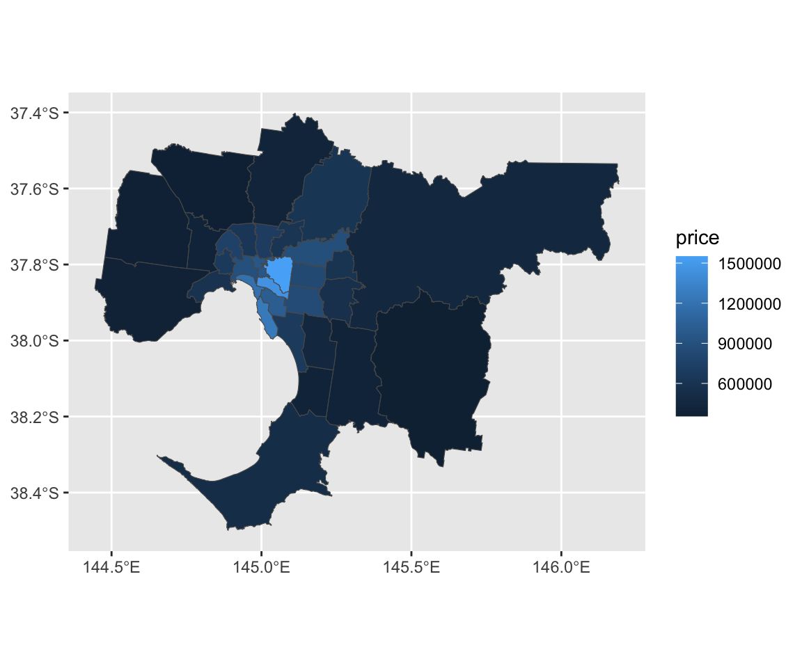
library(mapview)
mapView(gmel2, zcol = "price")
5 Reference
For more details of sf package, please see https://r-spatial.github.io/sf/articles/.