Extra 1: Visualisation of Spatial Data (4) – Data Wrangling using tidyr and dplyr
1 Introduction
In previous labs, we studied how to visualise the spatial objects. In this lab, we will study operations on the data frame (and therefore, sf object).
Two R packages (tidyr and dplyr) are designed to simplify the data cleaning and preparation.
2 tidyr
- Please study the tidyr package through the following
tutorial https://uc-r.github.io/tidyr. There are five commands
- %>%: the pipe operator
- gather
- spread
- separate
- unite
The function gather and spread has been retired, but it is still widely used in many books/blogs. The gather function is replaced by pivot_longer, and spread function is replaced by pivot_wider
library(tidyr)
relig_income
## # A tibble: 18 × 11
## religion `<$10k` `$10-20k` `$20-30k` `$30-40k` `$40-50k` `$50-75k` `$75-100k`
## <chr> <dbl> <dbl> <dbl> <dbl> <dbl> <dbl> <dbl>
## 1 Agnostic 27 34 60 81 76 137 122
## 2 Atheist 12 27 37 52 35 70 73
## 3 Buddhist 27 21 30 34 33 58 62
## 4 Catholic 418 617 732 670 638 1116 949
## 5 Don’t k… 15 14 15 11 10 35 21
## 6 Evangel… 575 869 1064 982 881 1486 949
## 7 Hindu 1 9 7 9 11 34 47
## 8 Histori… 228 244 236 238 197 223 131
## 9 Jehovah… 20 27 24 24 21 30 15
## 10 Jewish 19 19 25 25 30 95 69
## 11 Mainlin… 289 495 619 655 651 1107 939
## 12 Mormon 29 40 48 51 56 112 85
## 13 Muslim 6 7 9 10 9 23 16
## 14 Orthodox 13 17 23 32 32 47 38
## 15 Other C… 9 7 11 13 13 14 18
## 16 Other F… 20 33 40 46 49 63 46
## 17 Other W… 5 2 3 4 2 7 3
## 18 Unaffil… 217 299 374 365 341 528 407
## # ℹ 3 more variables: `$100-150k` <dbl>, `>150k` <dbl>,
## # `Don't know/refused` <dbl>relig_income %>% pivot_longer(!religion, names_to = "income", values_to = "count")## # A tibble: 180 × 3
## religion income count
## <chr> <chr> <dbl>
## 1 Agnostic <$10k 27
## 2 Agnostic $10-20k 34
## 3 Agnostic $20-30k 60
## 4 Agnostic $30-40k 81
## 5 Agnostic $40-50k 76
## 6 Agnostic $50-75k 137
## 7 Agnostic $75-100k 122
## 8 Agnostic $100-150k 109
## 9 Agnostic >150k 84
## 10 Agnostic Don't know/refused 96
## # ℹ 170 more rowsrelig_income %>% gather(key = income, value = count, -religion)## # A tibble: 180 × 3
## religion income count
## <chr> <chr> <dbl>
## 1 Agnostic <$10k 27
## 2 Atheist <$10k 12
## 3 Buddhist <$10k 27
## 4 Catholic <$10k 418
## 5 Don’t know/refused <$10k 15
## 6 Evangelical Prot <$10k 575
## 7 Hindu <$10k 1
## 8 Historically Black Prot <$10k 228
## 9 Jehovah's Witness <$10k 20
## 10 Jewish <$10k 19
## # ℹ 170 more rowsfish_encounters## # A tibble: 114 × 3
## fish station seen
## <fct> <fct> <int>
## 1 4842 Release 1
## 2 4842 I80_1 1
## 3 4842 Lisbon 1
## 4 4842 Rstr 1
## 5 4842 Base_TD 1
## 6 4842 BCE 1
## 7 4842 BCW 1
## 8 4842 BCE2 1
## 9 4842 BCW2 1
## 10 4842 MAE 1
## # ℹ 104 more rowsfish_encounters %>% pivot_wider(names_from = station, values_from = seen)## # A tibble: 19 × 12
## fish Release I80_1 Lisbon Rstr Base_TD BCE BCW BCE2 BCW2 MAE MAW
## <fct> <int> <int> <int> <int> <int> <int> <int> <int> <int> <int> <int>
## 1 4842 1 1 1 1 1 1 1 1 1 1 1
## 2 4843 1 1 1 1 1 1 1 1 1 1 1
## 3 4844 1 1 1 1 1 1 1 1 1 1 1
## 4 4845 1 1 1 1 1 NA NA NA NA NA NA
## 5 4847 1 1 1 NA NA NA NA NA NA NA NA
## 6 4848 1 1 1 1 NA NA NA NA NA NA NA
## 7 4849 1 1 NA NA NA NA NA NA NA NA NA
## 8 4850 1 1 NA 1 1 1 1 NA NA NA NA
## 9 4851 1 1 NA NA NA NA NA NA NA NA NA
## 10 4854 1 1 NA NA NA NA NA NA NA NA NA
## 11 4855 1 1 1 1 1 NA NA NA NA NA NA
## 12 4857 1 1 1 1 1 1 1 1 1 NA NA
## 13 4858 1 1 1 1 1 1 1 1 1 1 1
## 14 4859 1 1 1 1 1 NA NA NA NA NA NA
## 15 4861 1 1 1 1 1 1 1 1 1 1 1
## 16 4862 1 1 1 1 1 1 1 1 1 NA NA
## 17 4863 1 1 NA NA NA NA NA NA NA NA NA
## 18 4864 1 1 NA NA NA NA NA NA NA NA NA
## 19 4865 1 1 1 NA NA NA NA NA NA NA NAfish_encounters %>% spread(key = station, value = seen)## # A tibble: 19 × 12
## fish Release I80_1 Lisbon Rstr Base_TD BCE BCW BCE2 BCW2 MAE MAW
## <fct> <int> <int> <int> <int> <int> <int> <int> <int> <int> <int> <int>
## 1 4842 1 1 1 1 1 1 1 1 1 1 1
## 2 4843 1 1 1 1 1 1 1 1 1 1 1
## 3 4844 1 1 1 1 1 1 1 1 1 1 1
## 4 4845 1 1 1 1 1 NA NA NA NA NA NA
## 5 4847 1 1 1 NA NA NA NA NA NA NA NA
## 6 4848 1 1 1 1 NA NA NA NA NA NA NA
## 7 4849 1 1 NA NA NA NA NA NA NA NA NA
## 8 4850 1 1 NA 1 1 1 1 NA NA NA NA
## 9 4851 1 1 NA NA NA NA NA NA NA NA NA
## 10 4854 1 1 NA NA NA NA NA NA NA NA NA
## 11 4855 1 1 1 1 1 NA NA NA NA NA NA
## 12 4857 1 1 1 1 1 1 1 1 1 NA NA
## 13 4858 1 1 1 1 1 1 1 1 1 1 1
## 14 4859 1 1 1 1 1 NA NA NA NA NA NA
## 15 4861 1 1 1 1 1 1 1 1 1 1 1
## 16 4862 1 1 1 1 1 1 1 1 1 NA NA
## 17 4863 1 1 NA NA NA NA NA NA NA NA NA
## 18 4864 1 1 NA NA NA NA NA NA NA NA NA
## 19 4865 1 1 1 NA NA NA NA NA NA NA NA3 dplyr
- Please study the dplyr package through the following
tutorial https://cran.r-project.org/web/packages/dplyr/vignettes/base.html.
The tutorial includes a comparison betwwen commands of dplyr
and the equivalent from base R. The following commands are especially
useful
- arrange: Arrange rows by variables
- filter: Return rows with matching conditions
- mutate: Create or transform variables
- select: Select variables by name
- summarise: Reduce multiple values down to a single value
- The above commands only handle a data frame. For the operations in
two data frames. Please see Combine Data Sets of https://www.rstudio.com/wp-content/uploads/2015/02/data-wrangling-cheatsheet.pdf.
(This cheat sheet is also very useful as a future reference). In
particular, the following four commands:
- left_join
- right_join
- inner_join
- full_join
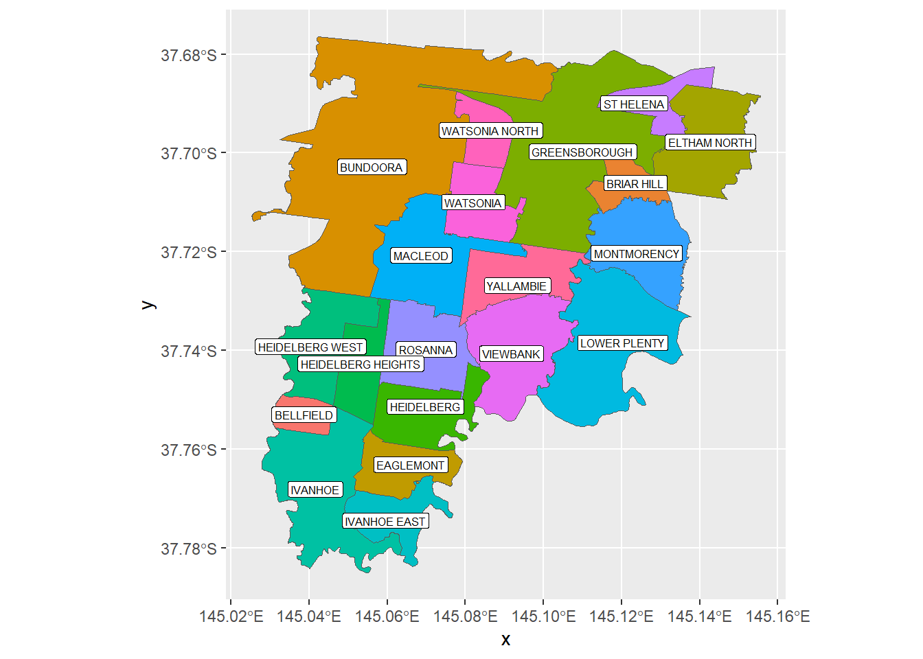
4 An Example
Suppose you want to plot all suburbs in City of Banyule. However, for suburbs shared with other LGAs, such as Bundoora, you want to plot the whole suburb, instead of the portion inside Banyule.
First, you can filter all these suburbs from VICSub. Here, I used the variable LC_PLY_PID instead of suburb names, because there are actually two Bellfield in Vitoria (and only one is in City of Banyule).
library(sf)
library(ggplot2)
library(dplyr)
load("datasets/BSub.Rdata")
VICSub = st_read(dsn="datasets/VICSub/VIC_LOCALITY_POLYGON_shp.shp", "VIC_LOCALITY_POLYGON_shp")
## Reading layer `VIC_LOCALITY_POLYGON_shp' from data source
## `/Users/tingjinc/Library/CloudStorage/OneDrive-TheUniversityofMelbourne/2_MAST90122/90122LabGit/datasets/VICSub/VIC_LOCALITY_POLYGON_shp.shp'
## using driver `ESRI Shapefile'
## Simple feature collection with 2973 features and 12 fields
## Geometry type: POLYGON
## Dimension: XY
## Bounding box: xmin: 140.9619 ymin: -39.13657 xmax: 149.9763 ymax: -33.98127
## Geodetic CRS: GDA2020VICSub <- st_transform(VICSub, 4326)
BSub2 = VICSub %>% filter(LC_PLY_PID %in% BSub$LC_PLY_PID)Afterward, you can visualise your results.
ggplot() + geom_sf(data = BSub2, aes(fill = VIC_LOCA_2)) +
  geom_sf_label(data = BSub2, aes(label = VIC_LOCA_2), size = 2.1) +
  theme(legend.position="none")