Geostatistical Data Example: Yearly Precipitation Anomaly Data
1 Dataset
library(sp)
library(ggplot2)
library(maps)
library(mapdata)
library(geoR)- Visualisation
- 936 weather stations across Great Plains that are north of 40 degrees latitude
- z: yearly precipitation anomaly in 1962
dfgeo = readRDS("datasets/dfgeo.rds")
states <- map_data("state")
plain <- subset(states, region %in% c("nebraska", "kansas", "colorado","wyoming",
                                      "south dakota", "north dakota", "montana",
                                      "iowa", "minnesota", "missouri"))
gg2 = ggplot(data = plain) +
  geom_polygon(aes(x = long, y = lat, group = group), fill = NA, color = "black") +
  coord_fixed(1.4)
gg2 + geom_point(data = dfgeo, aes(x = long, y = lat, color = z), size = 1)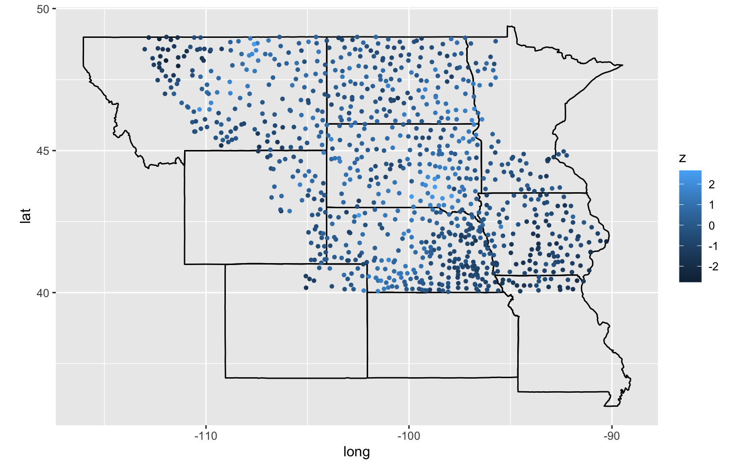
- About the distance
- 1 degree in latitude = 111 km
- 1 degree longitude at 45 degree latitude \(\approx\) 79 km
- If you want a more accurate distance than the above approximation, you need to use the function rdist.earth.
dfgeo$x = dfgeo$long * 79
dfgeo$y = dfgeo$lat * 111
The dataset is divided into two part, where dfgeo_train is used for modelling, and dfgeo_test is for kriging.
idx = seq(1, length(dfgeo$x), 5)
dfgeo_test = dfgeo[idx, ]
dfgeo_train = dfgeo[-idx,]
2 Model 1
- For Model 1: \[
Z(\mathbf{s}_i)=\mu+U(\mathbf{s}_i)+\nu(\mathbf{s}_i)
%\sum_{j=1}^p \beta_j d_j(x)+S(x)+Z(x) \]
- Constant mean: \(\mu\)
- Covariance function: exponential
2.1 Variogram and Initial Value for MLE
- The function variog is used to calculate the semivariogram
in our slides.
- option: “bin”
- max.dist: maximum distance for the semivariogram
dfgeodata =  as.geodata(dfgeo_train, coords.col=5:6, data.col=4, covar.col = 1:3)
plot(variog(dfgeodata, option="bin", max.dist=900),
     xlab = "h", ylab = "variogram")
## variog: computing omnidirectional variogram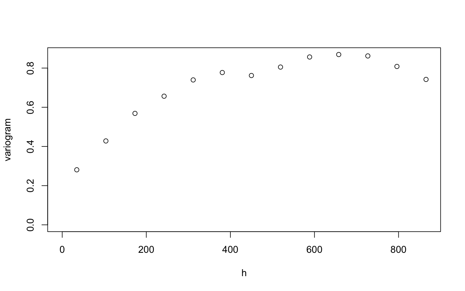
For the initial value, you first need to decide what type of covariance function you want to use. Here, we use the exponential covariance function (i.e., the matern class with \(\kappa = 0.5\).)
For the exponential covariance function, we choose the initial value \((\sigma^2, \phi, \tau^2) = (0.8, 200, 0.1)\). Since the line roughly follow the circles (the semivariograms), \((\sigma^2, \phi, \tau^2) = (0.8, 200, 0.1)\) is an appropriate initial value.
plot(variog(dfgeodata, option="bin", max.dist=900),
     xlab = "h", ylab = "variogram")
## variog: computing omnidirectional variogramlines.variomodel(seq(0, 900, l = 100),
cov.pars = c(0.8, 200),
cov.model = "mat", kap = 0.5, nug = 0.1)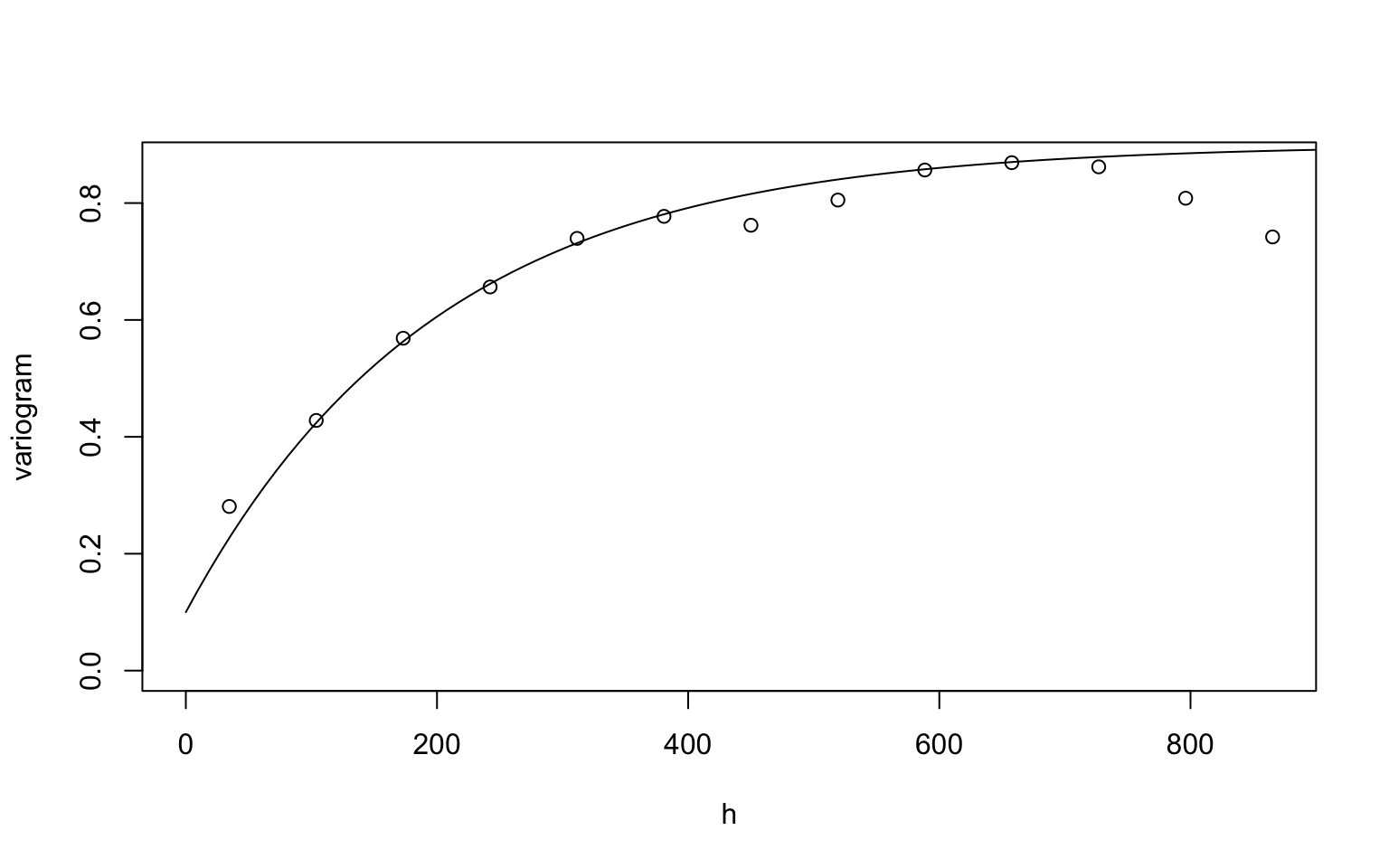
2.2 Model Specification
- The likfit function is used for MLE and REML for the geostatistical
model. To understand how the covariance function is specified, you first
need to know the default setting.
- cov.model= “matern”: matern class
- kappa = 0.5
- fix.kappa = TRUE: the kappa parameter is fixed at kappa = 0.5
- Therefore, if you do not write anything in the function, the default covariance function is the exponential covariance function, as shown in Model 1.
- Next, whether to estimate the nugget effect \(\tau^2\). The default setting is
- fix.nugget = FALSE: the nugget effect is estimated. If you want to fix the nugget effect, you need to write fix.nugget = TRUE.
- Therefore,
- nug = 0.1: the nugget effect is estimated, and the initial value is 0.1, as shown in Model 1.
- fix.nugget = FALSE, nug = 0.1: the same as the above.
- fix.nugget = TRUE, nug = 0.1: the nugget effect is fixed (NOT estimated) and the value is fixed at 0.1.
2.3 Model Fitting
## MLE: constant trend + exponential covariance function.
m1 = likfit(dfgeodata, ini = c(0.8, 200), nug = 0.1)## ---------------------------------------------------------------
## likfit: likelihood maximisation using the function optim.
## likfit: Use control() to pass additional
## arguments for the maximisation function.
## For further details see documentation for optim.
## likfit: It is highly advisable to run this function several
## times with different initial values for the parameters.
## likfit: WARNING: This step can be time demanding!
## ---------------------------------------------------------------
## likfit: end of numerical maximisation.First, check the convergence message, that is, $convergence = 0 indicates a successful convergence. (The likfit uses the optim funciton to minimize, that is, the message is the same as the message from the optim function)
m1$info.minimisation.function## $par
## [1] 152.6097186 0.1641731
##
## $value
## [1] 644.579
##
## $counts
## function gradient
## 24 24
##
## $convergence
## [1] 0
##
## $message
## [1] "CONVERGENCE: REL_REDUCTION_OF_F <= FACTR*EPSMCH"Second, whether the model improves over the linear model. At the bottom of the summary table, there are two rows: Maximised Likelihood (for the spatial model) and non spatial model.
2.4 The Results
Summary table includes most of information.
summary(m1)## Summary of the parameter estimation
## -----------------------------------
## Estimation method: maximum likelihood
##
## Parameters of the mean component (trend):
## beta
## -0.2176
##
## Parameters of the spatial component:
## correlation function: exponential
## (estimated) variance parameter sigmasq (partial sill) = 0.7136
## (estimated) cor. fct. parameter phi (range parameter) = 152.6
## anisotropy parameters:
## (fixed) anisotropy angle = 0 ( 0 degrees )
## (fixed) anisotropy ratio = 1
##
## Parameter of the error component:
## (estimated) nugget = 0.1172
##
## Transformation parameter:
## (fixed) Box-Cox parameter = 1 (no transformation)
##
## Practical Range with cor=0.05 for asymptotic range: 457.1779
##
## Maximised Likelihood:
## log.L n.params AIC BIC
## "-644.6" "4" "1297" "1316"
##
## non spatial model:
## log.L n.params AIC BIC
## "-968" "2" "1940" "1949"
##
## Call:
## likfit(geodata = dfgeodata, ini.cov.pars = c(0.8, 200), nugget = 0.1)- The \(\mu\) part
- in the summary table, it is denoted as *. In our example, \(\hat{\mu} = -0.2176\).
- It can also obtained by m1$beta
- The estimated asymptotic variance (matrix) is m1$beta.var
- A confidence interval or hypothesis testing can be conducted.
- For example, \(H_0 = 1\) versus \(H_1 \neq 1\). The test statistic = (m1$beta - 1)/sqrt(m1$beta.var) (approximately)\(\sim\) N(0,1).
m1$beta
# the estimated covariance matrix of beta.
m1$beta.var
# test statistic for the example
(m1$beta - 1)/sqrt(m1$beta.var)## [1] -0.2175513
## [1] 0.04546281
## [1] -5.710303- The \(\mathbf\theta\) part
- The estimate can be found in the summary table or via the codes below.
- The estimated asymptotic covariance matrix can be calculated using the formula in our slides, but it is not available through the likfit function.
# cov.pars
m1$cov.pars
# partial sill
m1$sigmasq
# the range parameter
m1$phi
# nugget
m1$nugget## [1] 0.7136275 152.6097186
## [1] 0.7136275
## [1] 152.6097
## [1] 0.1171584- Other information
# AIC of the model
AIC(m1)
# and others...
m1$practicalRange
logLik(m1)## [1] 1297.158
## [1] 457.1779
## 'log Lik.' -644.579 (df=4)3 Other Models
- For Model 2: \[
Z(\mathbf{s}_i)=\mu+U(\mathbf{s}_i)+\nu(\mathbf{s}_i)
%\sum_{j=1}^p \beta_j d_j(x)+S(x)+Z(x) \]
- Constant mean: \(\mu\)
- Covariance function: matern class with kappa = 1.5
Some key codes
## MLE: constant trend + matern class with kappa = 1.5
#plot(variog(dfgeodata, option="bin", max.dist=900),
# xlab = "h", ylab = "variogram")
#lines.variomodel(seq(0, 900, l = 100),
# cov.pars = c(0.8, 150),
# cov.model = "mat", kap = 1.5, nug = 0.1)
#m2 = likfit(dfgeodata, ini = c(0.8, 150), nug = 0.1, cov.model = "mat", kap = 1.5)
#m2$info.minimisation.function$convergence
#summary(m2)- For Model 3: \[
Z(\mathbf{s}_i)=\beta_0+x_1(\mathbf{s}_i)\beta_1+U(\mathbf{s}_i) +
\nu(\mathbf{s}_i)
%\sum_{j=1}^p \beta_j d_j(x)+S(x)+Z(x) \]
- Linear trend: \(x_1\) is the elevation
- Covariance function: exponential
The model is fitted using the REML method.
Some key codes
## The variogram, note ``trend = ~elev"
plot(variog(dfgeodata, option="bin", max.dist=900, trend = ~elev),
xlab = "h", ylab = "variogram")
lines.variomodel(seq(0, 900, l = 100),
                 cov.pars = c(0.8, 200),
                 cov.model = "mat", kap = 0.5, nug = 0.1)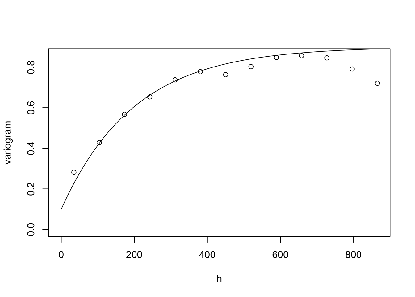
## variog: computing omnidirectional variogramm3 = likfit(dfgeodata, ini = c(0.8, 200), nug = 0.1, trend = ~ elev, lik.method = "REML")
summary(m3)## ---------------------------------------------------------------
## likfit: likelihood maximisation using the function optim.
## likfit: Use control() to pass additional
## arguments for the maximisation function.
## For further details see documentation for optim.
## likfit: It is highly advisable to run this function several
## times with different initial values for the parameters.
## likfit: WARNING: This step can be time demanding!
## ---------------------------------------------------------------
## likfit: end of numerical maximisation.
## Summary of the parameter estimation
## -----------------------------------
## Estimation method: restricted maximum likelihood
##
## Parameters of the mean component (trend):
## beta0 beta1
## -0.1025 -0.0003
##
## Parameters of the spatial component:
## correlation function: exponential
## (estimated) variance parameter sigmasq (partial sill) = 0.8754
## (estimated) cor. fct. parameter phi (range parameter) = 200
## anisotropy parameters:
## (fixed) anisotropy angle = 0 ( 0 degrees )
## (fixed) anisotropy ratio = 1
##
## Parameter of the error component:
## (estimated) nugget = 0.1227
##
## Transformation parameter:
## (fixed) Box-Cox parameter = 1 (no transformation)
##
## Practical Range with cor=0.05 for asymptotic range: 599.1464
##
## Maximised Likelihood:
## log.L n.params AIC BIC
## "-639.6" "5" "1289" "1312"
##
## non spatial model:
## log.L n.params AIC BIC
## "-960.9" "3" "1928" "1942"
##
## Call:
## likfit(geodata = dfgeodata, trend = ~elev, ini.cov.pars = c(0.8,
## 200), nugget = 0.1, lik.method = "REML")Asymptotic variance of \(\mathbf{\beta}\)
m3$beta.var## V1 V2
## V1 1.252390e-01 -5.861928e-05
## V2 -5.861928e-05 7.677583e-084 Kriging
- There are two key functions for the kriging
- krige.control: specify the parameter for kriging, no computing involved.
- krige.conv: to compute
- Usage
- krige.control(type.krige = “ok”, obj.model = NULL)
- Type of krige: “sk”, “ok” (default)
- sk: simple kriging
- ok: ordinary kriging and universal kriging
- obj.model: typically an output of likefit
- Usage
- krige.conv(geodata, locations, krige)
- geodata: the dataset for the model fitting
- locations: locations for predicting \(\mathbf s_0\), data.frame (can be multiple locations.)
- krige: output of krige.control.
4.1 Simple Kriging
kc1 = krige.control(obj.model = m1, type.krige = "SK")
m1krig_sk = krige.conv(dfgeodata, krige = kc1, locations = dfgeo_test[,5:6])
## krige.conv: model with constant mean
## krige.conv: Kriging performed using global neighbourhood4.2 Ordinary Kriging
kc2 = krige.control(obj.model = m1)
m1krig_ok = krige.conv(dfgeodata, krige = kc2, locations = dfgeo_test[,5:6])
## krige.conv: model with constant mean
## krige.conv: Kriging performed using global neighbourhood# The kriging predictors are the same
rbind(m1krig_sk$predict[1:5], m1krig_ok$predict[1:5])
# The kriging variances are different
rbind(m1krig_sk$krige.var[1:5], m1krig_ok$krige.var[1:5])## [,1] [,2] [,3] [,4] [,5]
## [1,] -0.05046874 -0.1163721 -0.9951614 0.5528769 -0.3275821
## [2,] -0.05046874 -0.1163721 -0.9951614 0.5528769 -0.3275821
## [,1] [,2] [,3] [,4] [,5]
## [1,] 0.3099821 0.2691624 0.3907208 0.3571768 0.3054627
## [2,] 0.3101195 0.2691632 0.3920374 0.3574023 0.30546434.3 Universal Kriging
- We need to provide \(x_1(\mathbf s_0),
\ldots, x_p(\mathbf s_0)\) for the function
- in function krige.control
- trend.d: specify data trend
- trend.l: specify prediction trend
We take Model 3 as an example
#kc3 = krige.control(type.krige = "ok", obj.model = m3, trend.d = ~elev, trend.l = ~dfgeo_test[,3])
#m3pred = krige.conv(dfgeodata, krige = kc3, locations = dfgeo_test[,5:6])