1 Test of CSR

1.1 Generate Poisson Process: HPP

library(spatstat)
data1 = rpoispp(lambda=100, win=owin(c(0,2),c(0,2)))
plot(data1, pch=46, cex =3)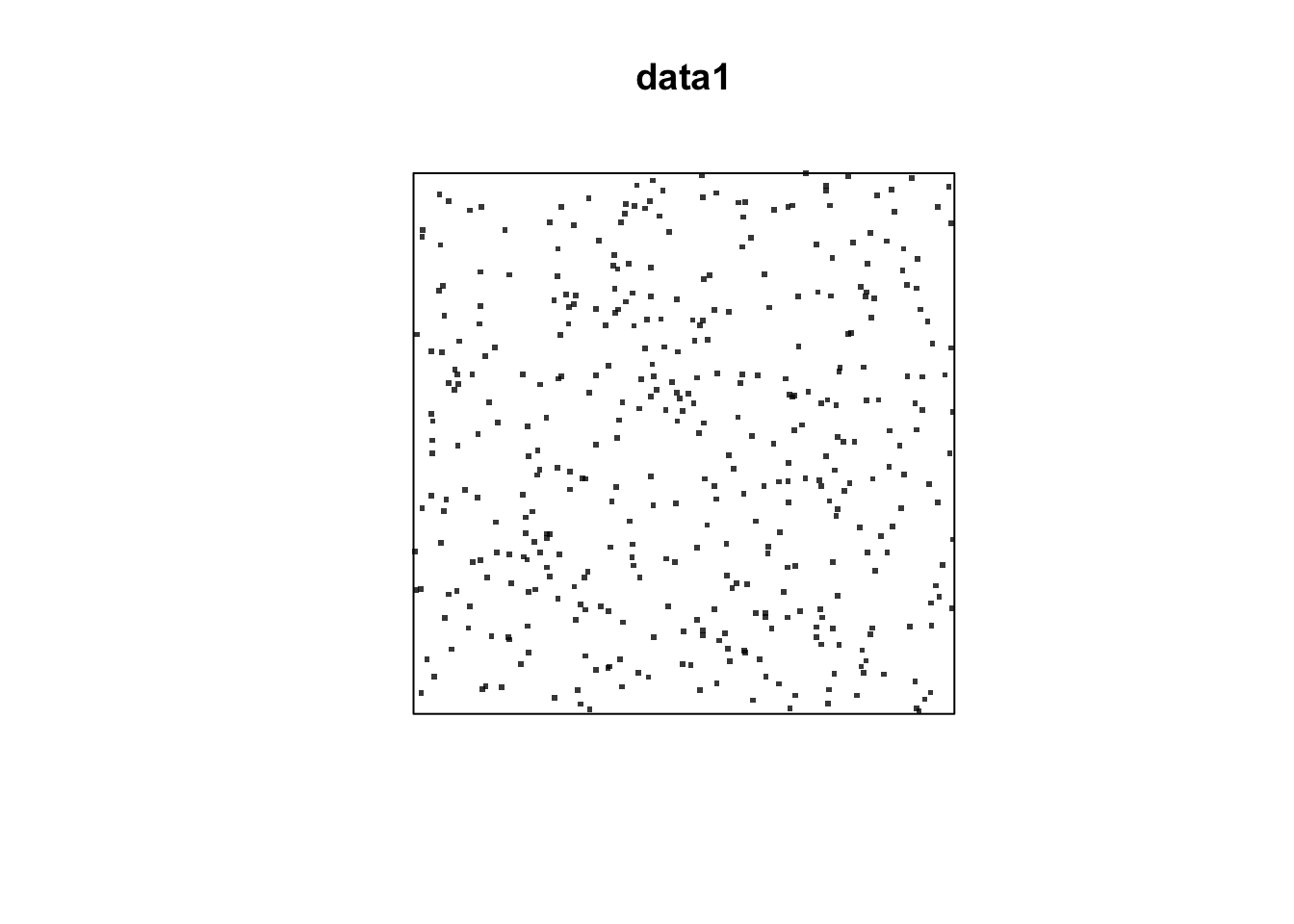

Argument:
- lambda=100: intensity function, NOT number of points
- win=owin(c(0,2),c(0,2)): spatial point process data will be generated in the domain D = [0,2]*[0,2].

Question: What is the expected number of events?

1.2 Quadrat test

Here, we will use R package spatstat

quadrat.test(data1, nx = 4, ny= 4, alternative = "two.sided", method = "Chisq")

## 
##  Chi-squared test of CSR using quadrat counts
## 
## data:  data1
## X2 = 15.02, df = 15, p-value = 0.9
## alternative hypothesis: two.sided
## 
## Quadrats: 4 by 4 grid of tiles

Argument:
- pp: the dataset must be a “ppp” class.
- nx=4, ny =4: number of block on x-axis and y-axis. Here, we have 4*4=16 blocks.
- alternative: alternative hypothesis. You can choose one of “two.sided”, “regular”, “clustered”.
- method: the method used to compute p-value. “Chisq” (analytical way), “MonteCarlo”

Since p-value is bigger than 0.05, we fail to reject \(H_0\).

1.3 Test: G Function

r=seq(0,sqrt(2), by=0.005)
Gtest=envelope(data1,fun=Gest, r=r, nrank=5, nsim=200)

## Generating 200 simulations of CSR  ...
## 1, 2, 3, 4.6.8.10.12.14.16.18.20.22.24.26.28.30.32.34
## .36.38.40.42.44.46.48.50.52.54.56.58.60.62.64.66.68.70.72.74
## .76.78.80.82.84.86.88.90.92.94.96.98.100.102.104.106.108.110.112.114
## .116.118.120.122.124.126.128.130.132.134.136.138.140.142.144.146.148.150.152.154
## .156.158.160.162.164.166.168.170.172.174.176.178.180.182.184.186.188.190.192.194
## .196.198.
## 200.
## 
## Done.

Argument:
- nsim: the number of simulated datasets
- nrank: similar to deciding the significance level
  - Note that (5+5)/200 = 0.05, and therefore, it is a similar to test at “significance level” = 0.05
  - That is, if you want to ensure \(\alpha\) (significance level), you need to set \((2nrank)/nsim = \alpha\).
- fun: Gest
- r: where the G function will be evaluated. (\(h\) in our slides.)

plot(Gtest)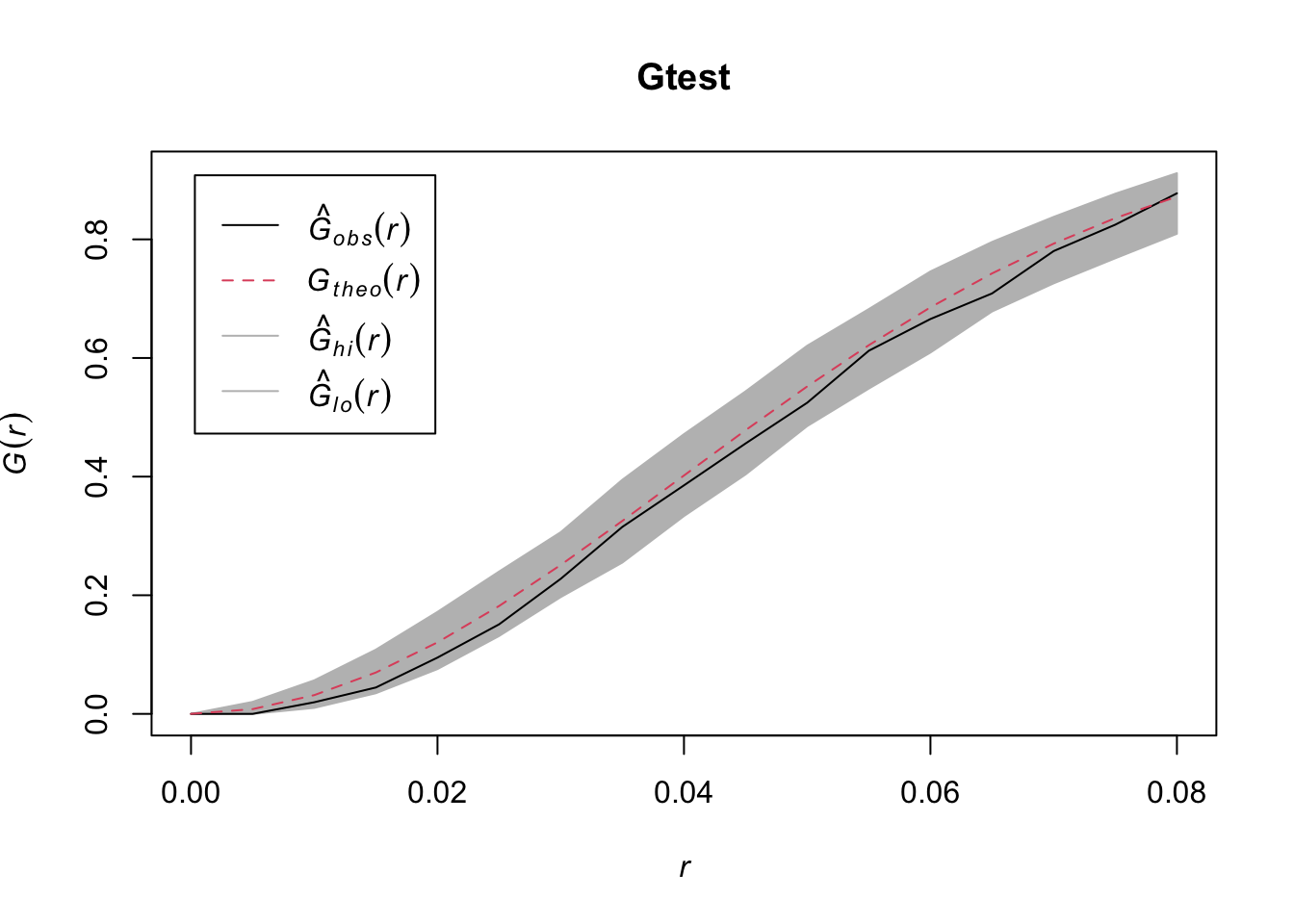

Question: What do you conclude from the above plot?

2 Spatial Point Models

2.1 Create IPP

# Inhomogeneous Poisson process in unit square
# with intensity lambda(x,y) = min(10 * exp(3*x), 100), where $s = (x, y)^T$
lamb = function(x,y) { 10 * exp( 3 * x)}
ipp = rpoispp(lambda=lamb, lmax=100) 
plot(ipp, pch=46, cex =3)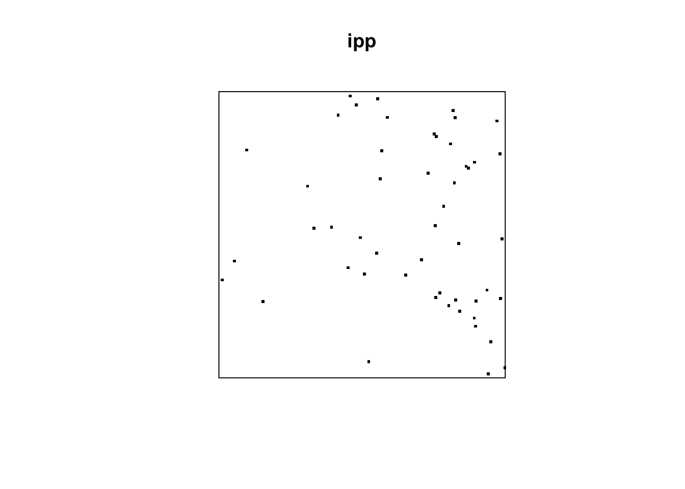

Here, lmax specifies the largest possible intensity. For example, when \(x=1\), we have \(10\exp(3x)=201\). However, since lmax = 100 is specified, the intensity will be 100. That is, we achieve “intensity lambda(x,y) = min(10 * exp(3*x), 100)“.

2.2 Create Neyman-Scott Process: clustered data pattern

set.seed(2025)
nclust <- function(x0, y0, radius, n) {
          return(runifdisc(n, radius, centre=c(x0, y0)))
            }
rNS = rNeymanScott(kappa=10, expand=0.1, 
                   rcluster = nclust, radius=0.1, n=10)
plot(rNS, pch=46, cex =3)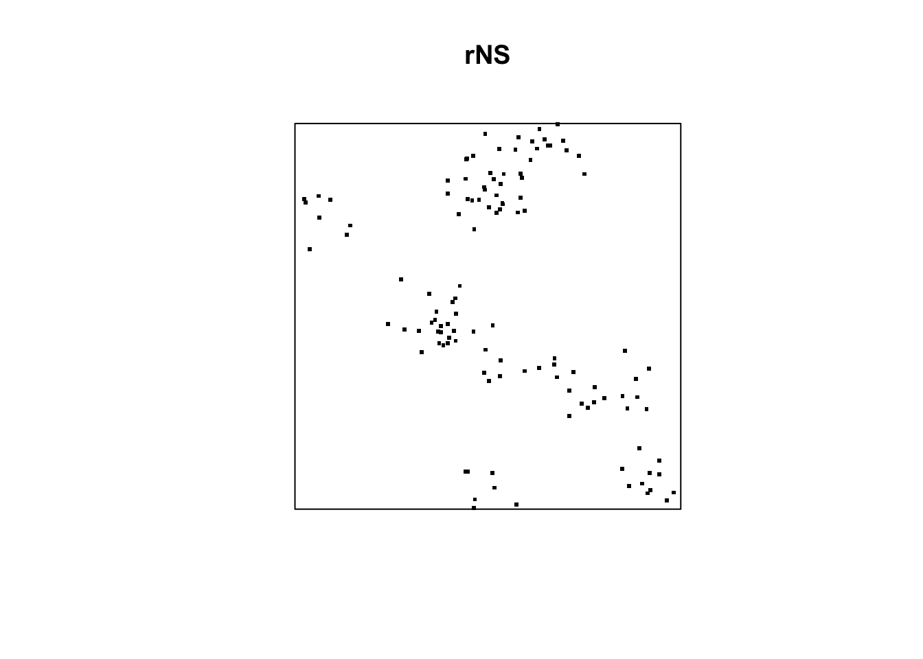

Argument:
- kappa: Intensity of the Poisson process for parent points (that is, \(\lambda\) in our slides) – step (i)
- expand: Size of the expansion of the simulation window for parent points – step (i)
- rcluster: step \((ii^*)--(iii^*)\): here runifdisc function is used.

About runifdisc function: runifdisc(n, radius)
- Generate a random point pattern containing \(n\) independent uniform random points in a circular disc.
- n: Number of offspring. Here, n=10 – in step \((ii^*)\).
- radius: Radius of the circle. radius = 0.1
- center: Coordinates of the center of the circle (that is, the location of the parent).

2.3 Create Matern I and Matern II: regular data pattern

par(mfrow=c(1,2))
matI = rMaternI(kappa = 10, r = 0.1)
plot(matI, main="", pch=46, cex =3)
matII = rMaternII(kappa = 10, r = 0.1)
plot(matII, main="", pch=46, cex =3)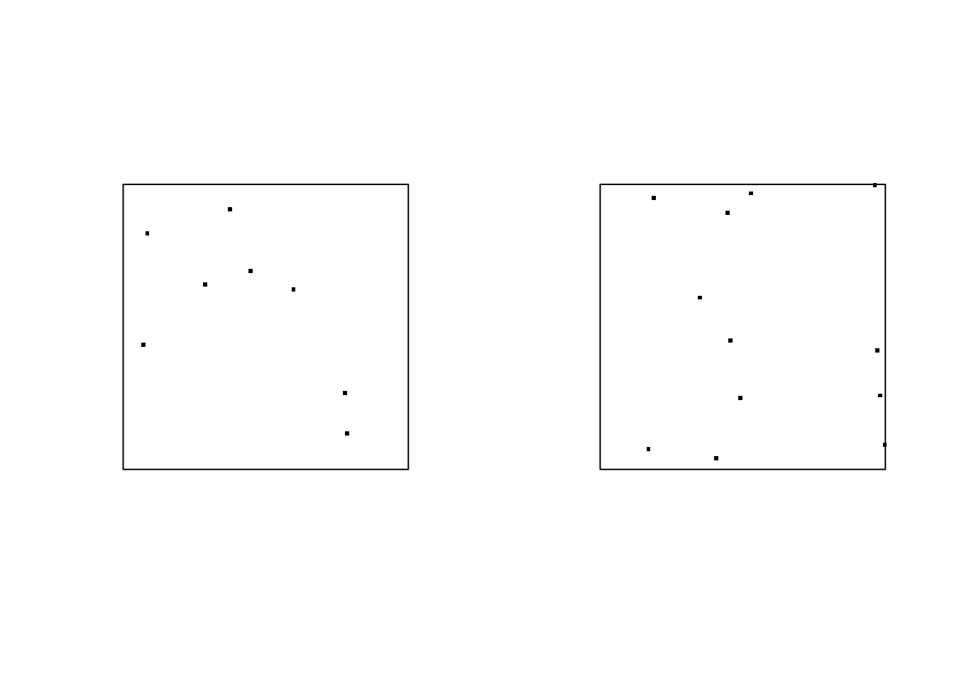

kappa: the intensity of the Poisson process (that is, \(\lambda\) in our slides).
r: Inhibition distance. (\(\delta\) in our slides)

3 Exercise

Two questions above.

Question: Can you test rNS data whether it follow clustered point pattern?

Week 4: Spatial Point Process – spatstat