1 Introduction

In Lab 11, we follow Lab 2.2 of Spatio-Temporal Statistics with R. You can download the electronic pdf through https://spacetimewithr.org/.
- In this document, I will only highlight some important points; that is, the visulization of spatio-temporal data.

2 Spatial Plots

First, we load the dataset.
- z: temperature (F)
- id: weather station ID.
- t: the same as the column day
- We do not really used column julian nor proc

library(dplyr)
library(tidyr)
library(ggplot2)
library(sf)


load("datasets/Tmax.Rdata")
head(Tmax)

##   julian year month day   id  z proc   lat       lon       date t
## 1 728050 1993     5   1 3804 82 Tmax 39.35 -81.43333 1993-05-01 1
## 2 728051 1993     5   2 3804 84 Tmax 39.35 -81.43333 1993-05-02 2
## 3 728052 1993     5   3 3804 79 Tmax 39.35 -81.43333 1993-05-03 3
## 4 728053 1993     5   4 3804 72 Tmax 39.35 -81.43333 1993-05-04 4
## 5 728054 1993     5   5 3804 73 Tmax 39.35 -81.43333 1993-05-05 5
## 6 728055 1993     5   6 3804 78 Tmax 39.35 -81.43333 1993-05-06 6

Next, the plot will be produced by package ggplot2. The new function here

We can also use sf object from Lab 5 and Lab 6 to achieve the same results. We transform the data to sf object using the function st_as_sf. Here, 4326 is WGS 84, which is the longitude and latitude.

Tmax_1 = Tmax %>% filter(t %in% c(1, 15, 30))  # extract data

state_sf = st_as_sf(maps::map("state", plot = FALSE, fill = TRUE), 
                        crs = st_crs(4326))
Tmax_1sf = st_as_sf(Tmax_1, coords = c("lon", "lat"), crs = st_crs(4326))

Next, visualise the data using geom_sf

NOAA_plot2 = ggplot() + geom_sf(data = state_sf) + 
  geom_sf(data = Tmax_1sf, aes(color = z)) + 
  coord_sf(xlim = c(-105, -75), ylim = c(25, 50)) + 
  scale_colour_gradientn(name = "degF", colours = terrain.colors(10)) + 
  facet_grid(~date)


NOAA_plot2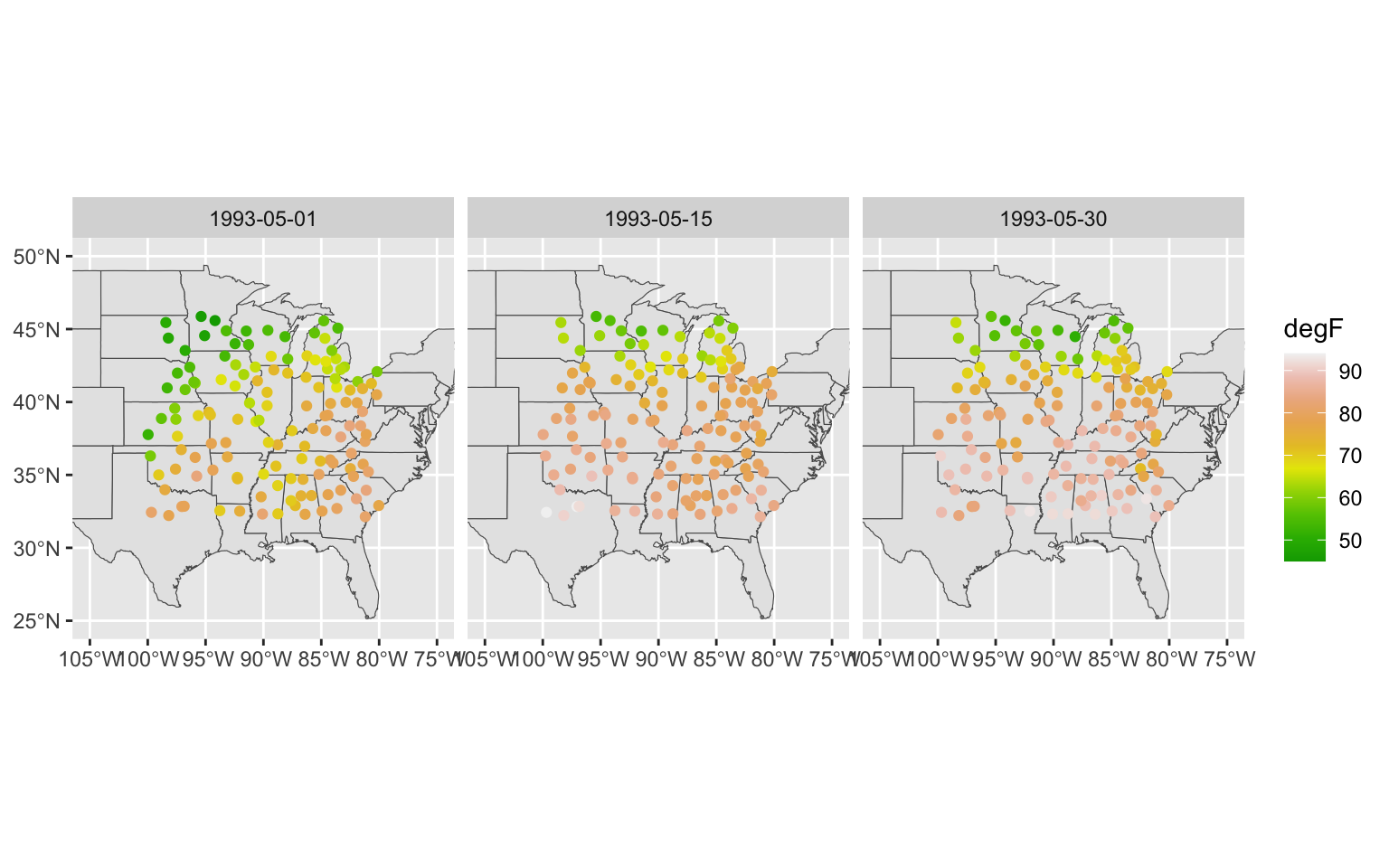

3 Time-Series Plots

First, we randomly select 10 station for visualization.

UIDs <- unique(Tmax$id)                     # extract IDs
UIDs_sub <- sample(UIDs, 10)                # sample 10 IDs
Tmax_sub <- filter(Tmax, id %in% UIDs_sub)  # subset data
head(Tmax_sub)

##   julian year month day    id  z proc  lat   lon       date t
## 1 728050 1993     5   1 13967 75 Tmax 35.4 -97.6 1993-05-01 1
## 2 728051 1993     5   2 13967 56 Tmax 35.4 -97.6 1993-05-02 2
## 3 728052 1993     5   3 13967 70 Tmax 35.4 -97.6 1993-05-03 3
## 4 728053 1993     5   4 13967 81 Tmax 35.4 -97.6 1993-05-04 4
## 5 728054 1993     5   5 13967 74 Tmax 35.4 -97.6 1993-05-05 5
## 6 728055 1993     5   6 13967 72 Tmax 35.4 -97.6 1993-05-06 6

Next, time-series is plotted.

## ------------------------------------------------------------------------
TmaxTS <- ggplot(Tmax_sub) +
    geom_line(aes(x = t, y = z)) +          # line plot of z against t
    facet_wrap(~id, ncol = 5) +             # facet by station
    xlab("Day number (days)") +             # x label
    ylab("Tmax (degF)") +                   # y label
    theme_bw() +                            # BW theme
    theme(panel.spacing = unit(1, "lines")) # facet spacing: the space between each subplots. 


TmaxTS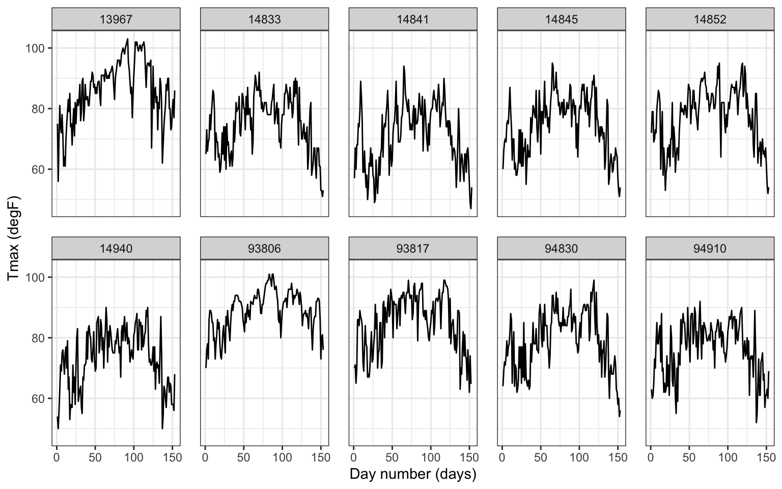

4 Spatio-Temporal Processess Animation

We have the locations of 10572 cases of non-specific gastro-intestinal disease in the county of Hampshire, UK, as reported to NHS Direct. Each location corresponds to the post-coded location of the residential address of the person making the call to NHS Direct.

The data include all such reported cases between 1 January 2001 and 31 December 2003. The unit of time is 1 day, with day 1 corresponding to 1 January 2001.

library(stpp)

## Warning in rgl.init(initValue, onlyNULL): X11 error: GLXBadContext

## Warning: 'rgl.init' failed, will use the null device.
## See '?rgl.useNULL' for ways to avoid this warning.

library(splancs)

data <- read.table("datasets/AEGISS_ixyt.dat", header = TRUE)
data <- data[order(data$t), ]
xy <- cbind(data$x, data$y)
poly <- scan("datasets/AEGISS_poly.dat", what = character())
poly <- as.numeric(poly)
poly <- matrix(poly, 120, 2, byrow = TRUE)

quartz() # open a new window and we can see the animation. Use windows() for windows system. 
xyt_data <- as.3dpoints(data$x[1:1000], 
                        data$y[1:1000], 
                        data$t[1:1000])
stpp::animation(xyt = xyt_data, 
                s.region = poly, 
                t.region = xyt_data[,3], runtime = 5)

Week 11: Visulization of Spatio-Temporal Data (Optional)

1 Introduction

2 Spatial Plots

3 Time-Series Plots

4 Spatio-Temporal Processess Animation