Week 6: Visualisation of Spatial Data (3) – Maps
1 Victoria maps: geom_sf
All datasets are read into as sf objects
library(ggplot2)
library(sf)
VICLGA = st_read(dsn = "datasets/VICLGA/VIC_LOCALITY_POLYGON_shp.shp", "VIC_LOCALITY_POLYGON_shp")
## Reading layer `VIC_LOCALITY_POLYGON_shp' from data source
## `/Users/tingjinc/Library/CloudStorage/OneDrive-TheUniversityofMelbourne/2_MAST90122/90122LabGit/datasets/VICLGA/VIC_LOCALITY_POLYGON_shp.shp'
## using driver `ESRI Shapefile'
## Simple feature collection with 92 features and 10 fields
## Geometry type: POLYGON
## Dimension: XY
## Bounding box: xmin: 140.9619 ymin: -39.13658 xmax: 149.9763 ymax: -33.98128
## Geodetic CRS: GDA94VICSub = st_read(dsn="datasets/VICSub/VIC_LOCALITY_POLYGON_shp.shp", "VIC_LOCALITY_POLYGON_shp")## Reading layer `VIC_LOCALITY_POLYGON_shp' from data source
## `/Users/tingjinc/Library/CloudStorage/OneDrive-TheUniversityofMelbourne/2_MAST90122/90122LabGit/datasets/VICSub/VIC_LOCALITY_POLYGON_shp.shp'
## using driver `ESRI Shapefile'
## Simple feature collection with 2973 features and 12 fields
## Geometry type: POLYGON
## Dimension: XY
## Bounding box: xmin: 140.9619 ymin: -39.13657 xmax: 149.9763 ymax: -33.98127
## Geodetic CRS: GDA2020First, we make sure that all sf objects has the same CRS
## Retrieve CRS
st_crs(VICLGA)
## Coordinate Reference System:
## User input: GDA94
## wkt:
## GEOGCRS["GDA94",
## DATUM["Geocentric Datum of Australia 1994",
## ELLIPSOID["GRS 1980",6378137,298.257222101,
## LENGTHUNIT["metre",1]]],
## PRIMEM["Greenwich",0,
## ANGLEUNIT["degree",0.0174532925199433]],
## CS[ellipsoidal,2],
## AXIS["geodetic latitude (Lat)",north,
## ORDER[1],
## ANGLEUNIT["degree",0.0174532925199433]],
## AXIS["geodetic longitude (Lon)",east,
## ORDER[2],
## ANGLEUNIT["degree",0.0174532925199433]],
## USAGE[
## SCOPE["Horizontal component of 3D system."],
## AREA["Australia including Lord Howe Island, Macquarie Island, Ashmore and Cartier Islands, Christmas Island, Cocos (Keeling) Islands, Norfolk Island. All onshore and offshore."],
## BBOX[-60.55,93.41,-8.47,173.34]],
## ID["EPSG",4283]]st_crs(VICSub)## Coordinate Reference System:
## User input: GDA2020
## wkt:
## GEOGCRS["GDA2020",
## DATUM["Geocentric Datum of Australia 2020",
## ELLIPSOID["GRS 1980",6378137,298.257222101,
## LENGTHUNIT["metre",1]]],
## PRIMEM["Greenwich",0,
## ANGLEUNIT["degree",0.0174532925199433]],
## CS[ellipsoidal,2],
## AXIS["geodetic latitude (Lat)",north,
## ORDER[1],
## ANGLEUNIT["degree",0.0174532925199433]],
## AXIS["geodetic longitude (Lon)",east,
## ORDER[2],
## ANGLEUNIT["degree",0.0174532925199433]],
## USAGE[
## SCOPE["Geodesy, cadastre, engineering survey, topographic mapping."],
## AREA["Australia including Lord Howe Island, Macquarie Island, Ashmore and Cartier Islands, Christmas Island, Cocos (Keeling) Islands, Norfolk Island. All onshore and offshore."],
## BBOX[-60.55,93.41,-8.47,173.34]],
## ID["EPSG",7844]]## Transform crs system to WGS84(epsg: 4326)
VICLGA <- st_transform(VICLGA, 4326)
VICSub <- st_transform(VICSub, 4326)
## Check CRS
#st_crs(VICLGA)
#st_crs(VICSub)Second, we want to obtain all suburbs in City of Banyule. Note that we already have all suburbs in Victoria, and we also know the boundary of City of Banyule from VICLGA. We only need to ``cut” all suburbs from VICSub using boundary of City of Banyule.
- One useful funciton in st_intersection in package
sf
- st_intersection(x, y)
- this function returns a geographic subset of an object x as specified by an extent object y
library(raster)
library(mapview)


## Obtain all suburbs in City of Banyule (including part of suburb)
i = which(VICLGA$VIC_LGA__3 == "BANYULE")
CMEL = VICLGA[i, ]
tmp = st_intersection(VICSub, CMEL)
tmp$VIC_LOCA_2
## [1] "MACLEOD" "HEIDELBERG WEST" "ROSANNA"
## [4] "RESERVOIR" "YALLAMBIE" "ALPHINGTON"
## [7] "BULLEEN" "VIEWBANK" "THORNBURY"
## [10] "ST HELENA" "HEIDELBERG" "EAGLEMONT"
## [13] "LOWER PLENTY" "ELTHAM NORTH" "ELTHAM"
## [16] "WATSONIA" "MONTMORENCY" "BRIAR HILL"
## [19] "BELLFIELD" "WATSONIA NORTH" "HEIDELBERG HEIGHTS"
## [22] "IVANHOE" "IVANHOE EAST" "KEW EAST"
## [25] "PRESTON" "TEMPLESTOWE LOWER" "TEMPLESTOWE"
## [28] "BUNDOORA" "GREENSBOROUGH" "BALWYN NORTH"The object tmp includes suburbs which is not in City of Banyule, such as Balwyn North. Here is a list of all suburbs in City of Banyule (https://en.wikipedia.org/wiki/City_of_Banyule). The reason for this is likely due to the different resolution and accuracy of shapefiles (VICSub and VICLGA).
Therefore, I will remove all the suburbs with a very small area (Here, the unit is square meter, and 10000 is small by suburb standards.)
## Obtain all suburbs in City of Banyule (including part of suburb)
tmp$area = st_area(tmp)
BSub = tmp[as.numeric(tmp$area) > 100000,]
mapView(BSub)
save(BSub, file = "datasets/BSub.Rdata") There are major activity centres. According to the goverment, These are places that provide a suburban focal point for services, employment, housing, public transport and social interaction. They have different attributes and provide different functions, with some serving larger subregional catchments. Plan Melbourne identifies 121 existing and future Major Activity Centres across Melbourne.
Suppose we want to obtain all major activity centres in the City of Banyule. Note these acitivity centres are represented as points
centres = st_read(dsn = "datasets/PlanMel/Activity Centres/ActivityCentrePoints_font_point.shp",
                 "ActivityCentrePoints_font_point")
## Reading layer `ActivityCentrePoints_font_point' from data source
## `/Users/tingjinc/Library/CloudStorage/OneDrive-TheUniversityofMelbourne/2_MAST90122/90122LabGit/datasets/PlanMel/Activity Centres/ActivityCentrePoints_font_point.shp'
## using driver `ESRI Shapefile'
## Simple feature collection with 133 features and 6 fields
## Geometry type: POINT
## Dimension: XYZ
## Bounding box: xmin: 144.5651 ymin: -38.35552 xmax: 145.4818 ymax: -37.41308
## z_range: zmin: 0 zmax: 0
## Geodetic CRS: GDA94centres <- st_transform(centres, 4326)
## obtain all centres within the City of Banyule (CMEL)
tmp = st_within(centres, CMEL, sparse = F)
Bcen = centres[tmp[,1],]
library(ggplot2)
library(sf)
ggplot() + geom_sf(data = BSub, aes(fill = VIC_LOCA_2)) +
geom_sf_label(data = BSub, aes(label = VIC_LOCA_2), size = 2.1) +
geom_sf(data = Bcen, size = 4) + theme(legend.position="none")## Warning in st_point_on_surface.sfc(sf::st_zm(x)): st_point_on_surface may not
## give correct results for longitude/latitude data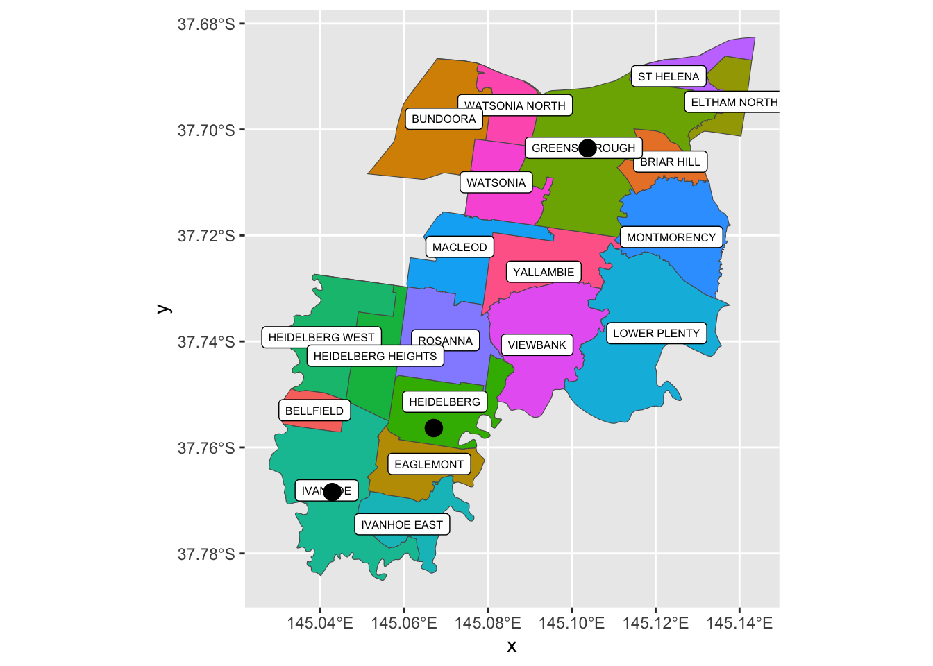
Suppose you also want to draw major roads in City of Banyule. The shapefile of all roads are in the folder VMTRANS. Here, we want to draw all roads with Road Class = 0, 1, 2. (I do not know what Road Class really means here, but it appears the smaller number indicates a more important road.)
road = st_read(dsn = "datasets/VMTRANS/TR_ROAD.shp", "TR_ROAD")## Reading layer `TR_ROAD' from data source
## `/Users/tingjinc/Library/CloudStorage/OneDrive-TheUniversityofMelbourne/2_MAST90122/90122LabGit/datasets/VMTRANS/TR_ROAD.shp'
## using driver `ESRI Shapefile'
## Simple feature collection with 7131 features and 70 fields
## Geometry type: LINESTRING
## Dimension: XY
## Bounding box: xmin: 145.0287 ymin: -37.78299 xmax: 145.1478 ymax: -37.68205
## Geodetic CRS: GDA2020road <- st_transform(road, 4326)
## You can see all roads in Banyule
#mapView(road)
## We only draw road with CLASS_CODE = 0, 1, 2
highway = road[road$CLASS_CODE < 3,]
#mapView(highway)
## Now add all together
ggplot() + geom_sf(data = BSub, color = "gray") +
geom_sf(data = Bcen, size = 4) +
geom_sf(data = highway, aes(color = as.factor(CLASS_CODE)), lwd = 1.5) 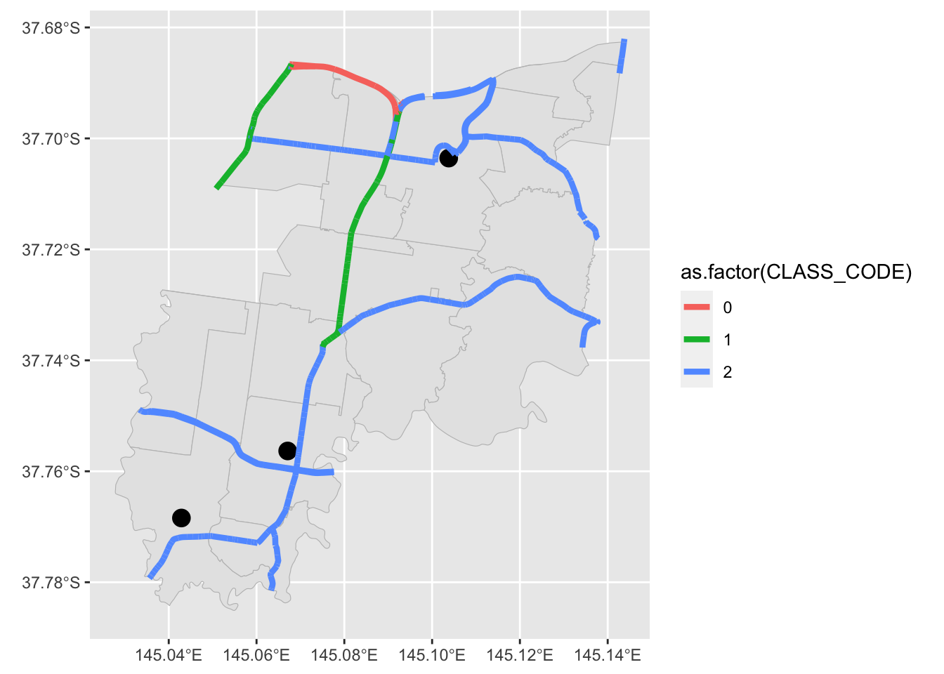
2 R package maps and mapdata
R package maps and mapdata provide some maps. They are not in sf format. To convert map data to sf, use following codes
state_sf = sf::st_as_sf(maps::map("state", plot = FALSE, fill = TRUE))

ggplot() + geom_sf(data = state_sf)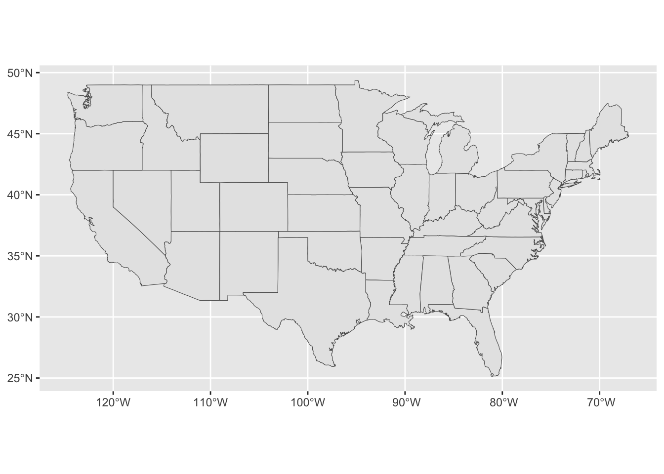
If you want to plot directly using geom_polygon, see Extra3.