1 USA map

R package maps and mapdata provide some maps. We will use them for the USA map

library(ggplot2)
library(maps)
library(mapdata)
library(sp)
usa <- map_data("usa")
dim(usa)

## [1] 7243    6

head(usa)

##        long      lat group order region subregion
## 1 -101.4078 29.74224     1     1   main      <NA>
## 2 -101.3906 29.74224     1     2   main      <NA>
## 3 -101.3620 29.65056     1     3   main      <NA>
## 4 -101.3505 29.63911     1     4   main      <NA>
## 5 -101.3219 29.63338     1     5   main      <NA>
## 6 -101.3047 29.64484     1     6   main      <NA>

tail(usa)

##           long      lat group order         region subregion
## 7247 -122.6187 48.37482    10  7247 whidbey island      <NA>
## 7248 -122.6359 48.35764    10  7248 whidbey island      <NA>
## 7249 -122.6703 48.31180    10  7249 whidbey island      <NA>
## 7250 -122.7218 48.23732    10  7250 whidbey island      <NA>
## 7251 -122.7104 48.21440    10  7251 whidbey island      <NA>
## 7252 -122.6703 48.17429    10  7252 whidbey island      <NA>

First, we plot usa map

library(gridExtra)
gg0 = ggplot() + geom_polygon(data = usa, aes(x=long, y = lat, group = group)) + 
  coord_quickmap()
gg1 <- ggplot() + 
  geom_polygon(data = usa, aes(x=long, y = lat, group = group), fill = "violet", color = "blue") + 
  coord_quickmap()
labs <- data.frame(
  long = c(-122.064873, -122.306417),
  lat = c(36.951968, 47.644855),
  names = c("SWFSC-FED", "NWFSC"),
  stringsAsFactors = FALSE
)  
gg2 = gg1 + 
  geom_point(data = labs, aes(x = long, y = lat), color = "yellow", size = 2)

grid.arrange(gg0, gg1, gg2, nrow = 1)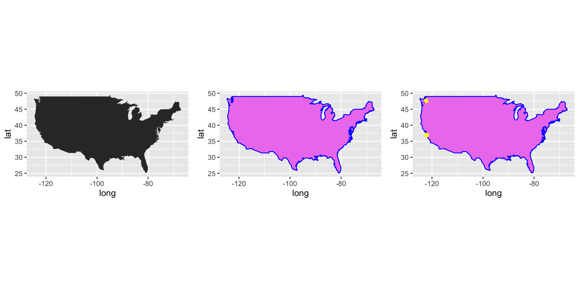

Key points
- “group = group” is essential, you can try code without the group argument.
- coord_quickmap(): one degree longitude is not the same distance as one degree latitude. For the latitude at 40, it is about \(1/cos(2\pi/9) \approx 1.3\) of that of the longitude. coord_quickmap() can fix this automatically, see Chpater 9.7 of RDS book (https://r4ds.hadley.nz/layers#coordinate-systems).
- the two dots represents two cities.

2 US state

### Draw plots for all USA States
states <- map_data("state")
ggplot(data = states) + 
  geom_polygon(aes(x = long, y = lat, fill = region, group = group), color = "white") + 
  coord_quickmap() + guides(fill=FALSE)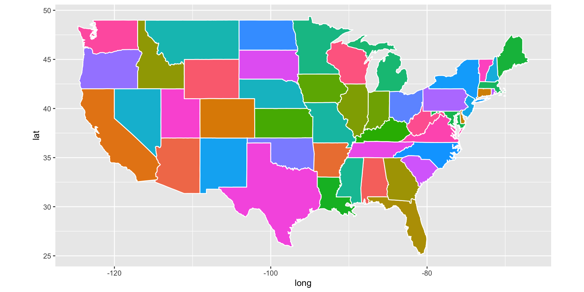

### Draw a subset of USA states
### Use function subset to select states. 
west_coast <- subset(states, region %in% c("california", "oregon", "washington"))
ggplot(data = west_coast) + 
  geom_polygon(aes(x = long, y = lat, group = group), fill = "palegreen", color = "red") + 
  coord_quickmap()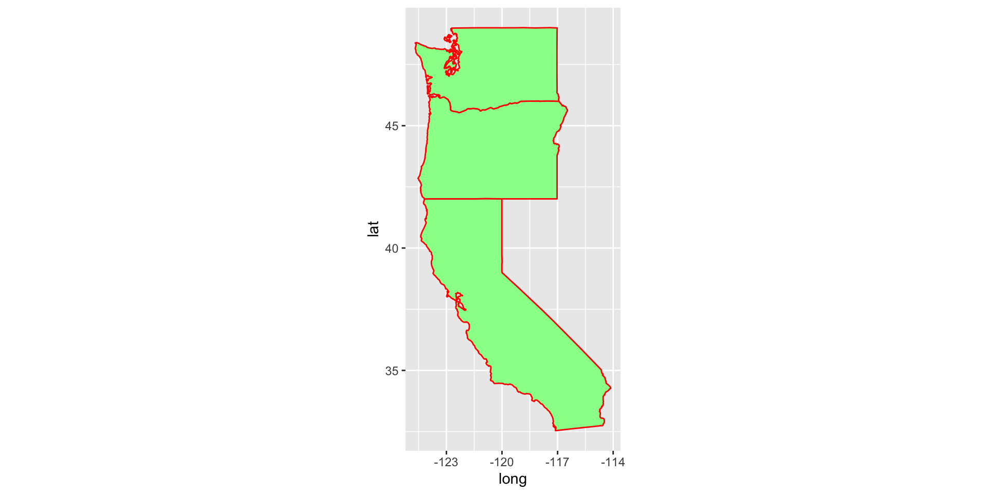

Can you tell the difference between color and fill argument?

Geom_polygon – Maps

1 USA map

2 US state