Extra 2: Spatial Data Classes – package sp
1 Introduction
- In this lab, you will learn
- Create different type of spatial objects
- Some basic property and manipulation of these spatial objects
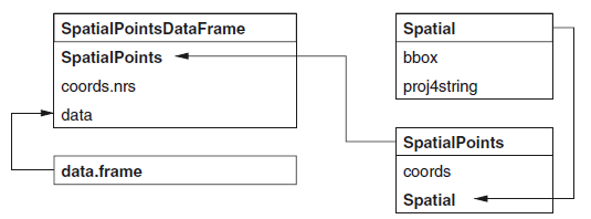
2 SpatialPointsDataFrame Class
Information of spatial class can be found in class notes: Chpater 3–Visualisation.
The diagram will help
2.1 Create Spatial Class
- For Spatial class, we will need two components
- bbox: it is the domain of spatial objects. In the following example, the domain is \([0,1]\times [0,1]\).
- CRS: coordinate reference sytem (See Cp3 for more details). In the following example, the CRS is WGS84.
library(sp)
m=matrix(c(0,0,1,1),ncol=2, dimnames=list(NULL, c("min","max")))
crs=CRS(projargs="+proj=longlat +ellps=WGS84")
S=Spatial(bbox=m, proj4string=crs)
At this stage, nothing is plotted yet. Next, we will add points through SpatialPoints class
2.2 Create SpatialPoints Class
Recall SpatialPoints = Spatial + coords. We would like to add 4 points: \((1,1), (2,2), (3,3), (4,4)\). It can be achieved through coords = loccords, where loccords is a matrix containing locations (you can use other names if you want.)
lcoords=matrix(rep(1:4,each=2),ncol=2,byrow=T)    ## coords
SP=SpatialPoints(coords = lcoords,bbox = m, proj4string = crs)

## Access the elements
bbox(SP)
## min max
## [1,] 0 1
## [2,] 0 1proj4string(SP)## [1] "+proj=longlat +ellps=WGS84 +no_defs"SP@coords## coords.x1 coords.x2
## [1,] 1 1
## [2,] 2 2
## [3,] 3 3
## [4,] 4 4SP@bbox## min max
## [1,] 0 1
## [2,] 0 1SP@proj4string## Coordinate Reference System:
## Deprecated Proj.4 representation: +proj=longlat +ellps=WGS84 +no_defs
## WKT2 2019 representation:
## GEOGCRS["unknown",
## DATUM["Unknown based on WGS84 ellipsoid",
## ELLIPSOID["WGS 84",6378137,298.257223563,
## LENGTHUNIT["metre",1],
## ID["EPSG",7030]]],
## PRIMEM["Greenwich",0,
## ANGLEUNIT["degree",0.0174532925199433],
## ID["EPSG",8901]],
## CS[ellipsoidal,2],
## AXIS["longitude",east,
## ORDER[1],
## ANGLEUNIT["degree",0.0174532925199433,
## ID["EPSG",9122]]],
## AXIS["latitude",north,
## ORDER[2],
## ANGLEUNIT["degree",0.0174532925199433,
## ID["EPSG",9122]]]]## plot
plot(SP)
- Question: There are supposed to be four points.
- Why are you only seeing one?
- Do you know how to fix it (hint: adjust bbox)
2.3 Create SpatialPointsDataFrame Class
Recall SpatialPointsDataFrame = SpatialPoints + data.frame
Imagine we would like to add attribute to SpatialPoints. The way to achieve this is through data.frame. For example, we would like to assign attribute \(Z(s_1)=1.1\), \(Z(s_2)=1.2\), \(Z(s_3)=1.6\) and \(Z(s_4)=2.1\).
The argument coords.nrs is optional, and will not be used in this subject.
names=c("a","b","c","d")
df = data.frame(z=c(1.1,1.2,1.6,2.1), row.names=names)
m = matrix(c(0,0,5,5),ncol=2, dimnames=list(NULL, c("min","max")))
SP@bbox = m
SPDF = SpatialPointsDataFrame(SP,data=df)

## Access the elements
SPDF@data
## z
## a 1.1
## b 1.2
## c 1.6
## d 2.1## Plot: location with value
## Note here that you need to write "z" which is the same name you defined in df.
spplot(SPDF,zcol="z")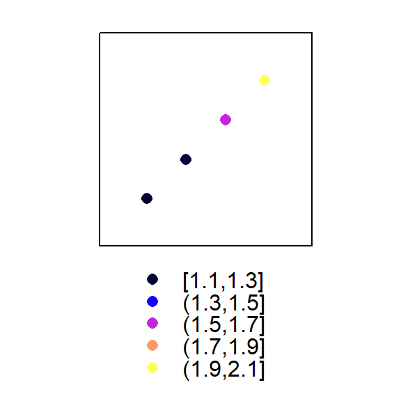
## Another way to create SpatialPointsDataFrame (directly from a data.frame)
SPDF2 = data.frame(name = names, x = lcoords[,1], y = lcoords[,2], value = df )
coordinates(SPDF2) = ~x+y
class(SPDF2)
## [1] "SpatialPointsDataFrame"
## attr(,"package")
## [1] "sp"proj4string(SPDF2) <- CRS("+proj=longlat +datum=WGS84") ## Add CRS3 SpatialPolygonsDataFrame
Due to time constrain, I will not talk about spatiallines class. Instead, I will focus on SpatialPolygonsDataFrame.
First, the diagram
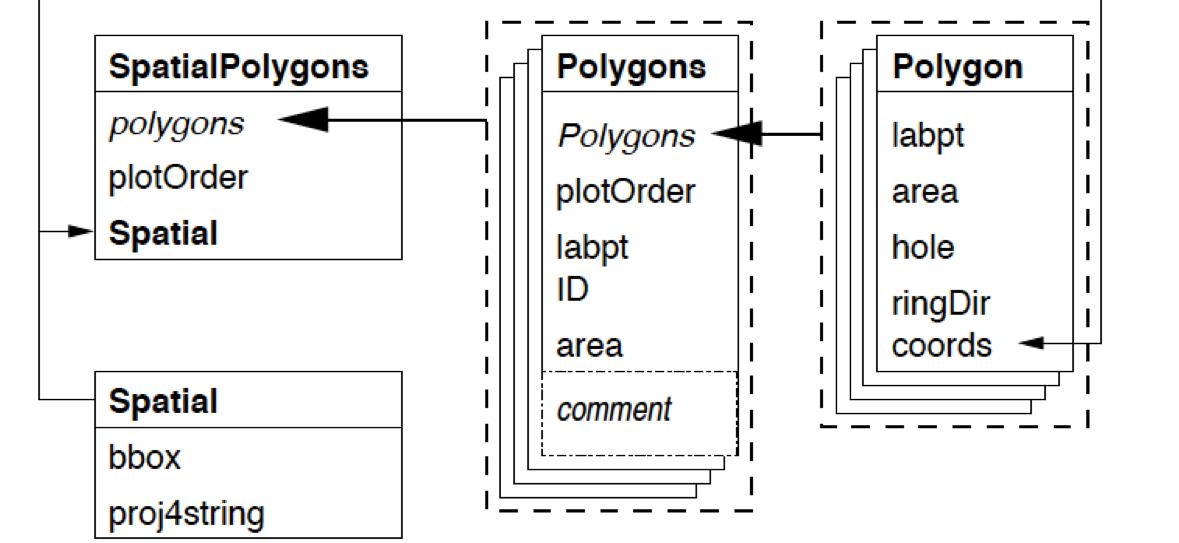
3.1 Create Polygon
Here, we will create Polygon class. For example, Sr1 has the vertices \((2,2)\), \((4,3)\), \((4,5)\) and \((1,4)\). Note that \((2,2)\) needs to be written twice, since it is both the starting vertex and the ending vertex.
#getClass("Polygon")
Sr1 = Polygon(cbind(c(2,4,4,1,2),c(2,3,5,4,2)))
Sr2 = Polygon(cbind(c(5,4,2,5),c(2,3,2,2)))
Sr3 = Polygon(cbind(c(4,4,5,10,4),c(5,3,2,5,5)))
Sr4 = Polygon(cbind(c(5,6,6,5,5),c(4,4,3,3,4)), hole = TRUE)
3.2 Create Polygons
A Polygons can contain any number of Polygon (including only 1 Polygon).
Why do we need polygons? Imagine you want to draw world map. Each Polygons can represent a country, while a Polygon cannot. For example, New Zealand comprises two major islands, and you need two polygons, which is a Polygons.
#getClass("Polygons")
Srs1 = Polygons(list(Sr1), "s1")
Srs2 = Polygons(list(Sr2), "s2")
Srs3 = Polygons(list(Sr3, Sr4), "s3/4")
3.3 Create SpatialPolygons
#getClass("SpatialPolygons")
SpP = SpatialPolygons(list(Srs1,Srs2,Srs3), 1:3)
plot(SpP, col = 1:3, bg="yellow")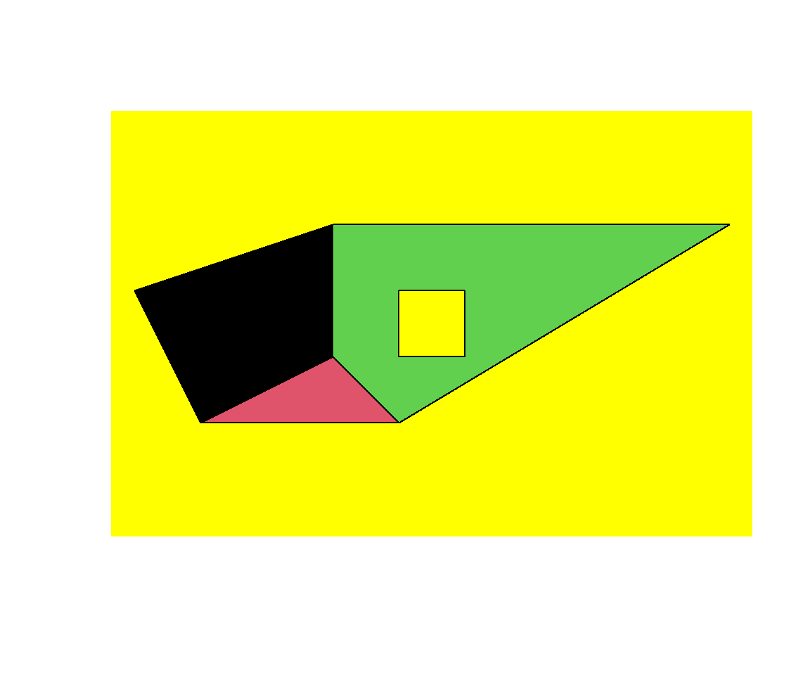 Note that there is a hole in one of Polygons
3.4 Create SpatialPolygonsDataFrame
#getClass("SpatialPolygons")
df = data.frame(z1 = c(1.2,1.3,1.6), z2 = c(2.2,2.8,3.9), row.names = row.names(SpP))
SpPDF = SpatialPolygonsDataFrame(Sr = SpP, data = df)
spplot(SpPDF, zcol = "z1")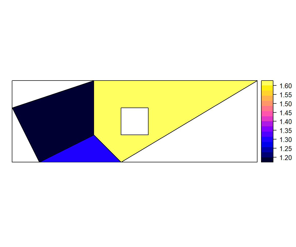 The argument “row.names = row.names(SpP)” is needed.
4 Review: Key Functions
- Create spatial objects
- Spatial
- SpatialPoints, SpatialPointsDataFrame
- SpatialPolygons, SpatialPolygonsDataFrame
- Visualization
- spplot
5 Further Study
Study vector data manipulation(https://rspatial.org/raster/spatial/7-vectmanip.html). Here, vector data is referring to SpatialPolygonsDataFrame.
6 References
- For more information, please see (Not required to read, and treat
the following materials as reference. )
- Classes and Methods for Spatial Data: the sp Package (https://cran.r-project.org/web/packages/sp/vignettes/intro_sp.pdf)
- Introduction to visualising spatial data in R (https://cran.r-project.org/doc/contrib/intro-spatial-rl.pdf)
- Spatial data manipulation (https://rspatial.org/raster/spatial/index.html)